Advanced High-Precision Publication-Ready Graphics Suite
plot_agri_graphics.RdThe `plot_agri_graphics` function serves as the unified visualization hub for the AgriDataTools package. It handles basic statistical diagnostics (residuals, correlations) alongside modern publication-grade graphical representations for mean performance, PCA space, hierarchical dendrograms, and path analysis direct effects.
Usage
plot_agri_graphics(
  type,
  payload,
  trait_name = "Target Character Matrix",
  reporting_level = 2,
  num_clusters = 4
)
Arguments
- type
A single character string specifying the target chart module:
"residual","correlation","mean","pca","cluster", or"path".- payload
A structured analysis
listderived from computational engines (e.g.,compute_lsd,analyze_pca,analyze_clustering,compute_path_analysis).- trait_name
A character string defining the target phenotypic trait title label. Used primarily in
"mean"and"path"layouts.- reporting_level
An integer vector flag defining console trace settings:
0for silent,1for structural updates, and2for exhaustive analytical tracing. Defaults to2.- num_clusters
An integer specifying the number of cluster groups to color in the circular dendrogram module. Defaults to
4.
Value
Invisibly returns a logical scalar TRUE upon successful execution.
This function is primarily invoked for its side effect of rendering publication-grade
graphical plots (e.g., residual diagnostic plots, correlation heatmaps, mean performance
barcharts, PCA biplots, circular dendrograms, or path analysis plots) to the active
graphics device.
Details
Visualizing high-dimensional screening metrics across diverse lines or cultivars requires balancing diagnostic model validation checks with advanced multivariate aesthetics. This engine supports base diagnostic rendering as well as optimized ggplot2 geometries featuring dynamic color palettes, non-overlapping labels, and geometric layout vector mapping fields.
Examples
data(gv_data, package = "AgriDataTools")
traits <- c("PH", "SL", "PL", "NOT", "NOSS", "TGW", "GYPM")
# Define custom mapping or number of clusters beforehand
k_groups <- 4
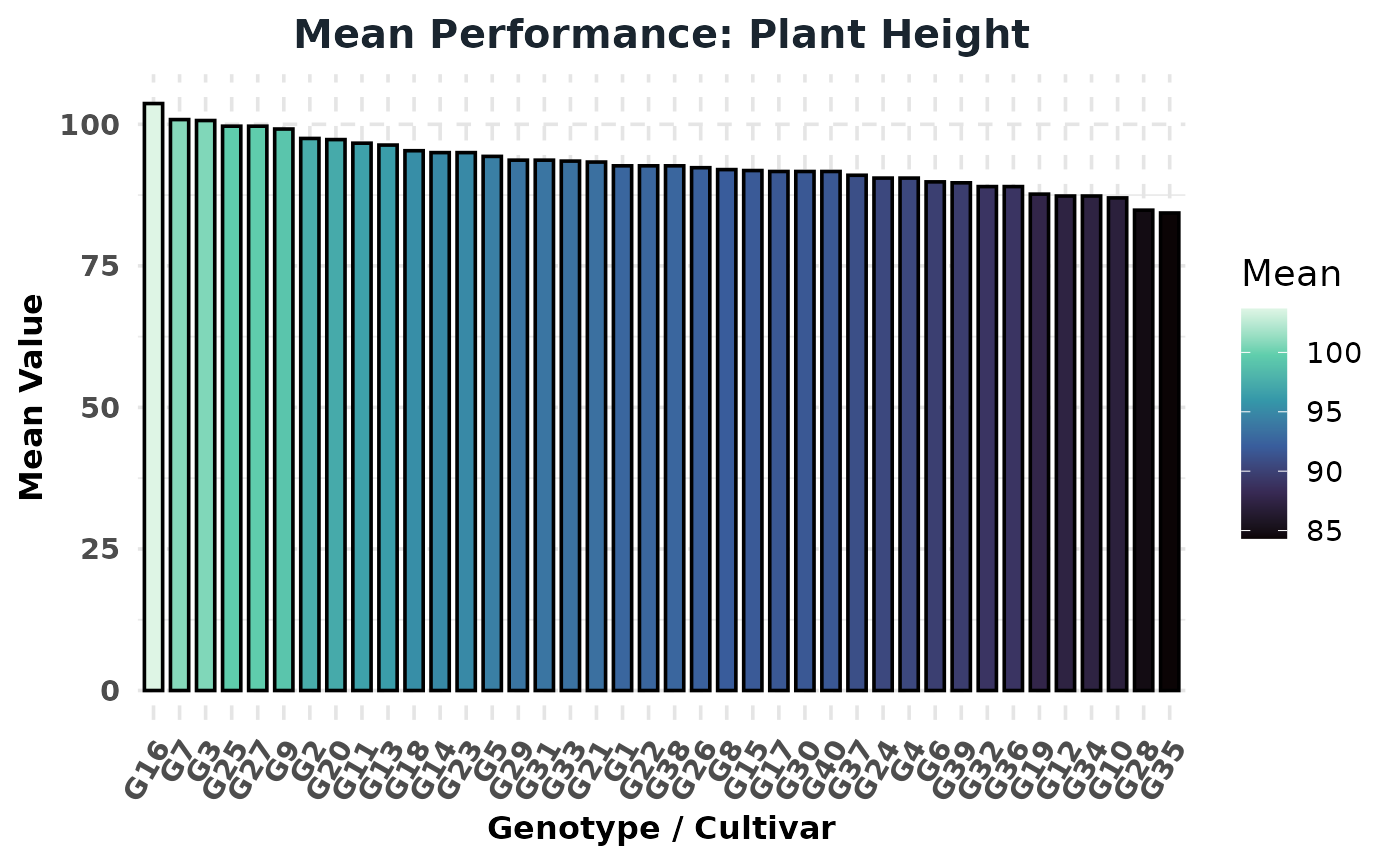
# 1. Mean performance: Genotypic performance with LSD
reps <- length(unique(gv_data$Replication))
fit <- aov(PH ~ Genotype + Replication, data = gv_data)
m_anova <- list(anova_table = data.frame(
Source = c("Genotype", "Replication", "Error"),
Df = summary(fit)[[1]]$Df,
MS = summary(fit)[[1]][[3]]
))
lsd_res <- compute_lsd(gv_data, "PH", m_anova, reps)
plot_agri_graphics(type = "mean", payload = lsd_res,
trait_name = "Plant Height")
#> =====================================================================================
#> AGRIDATATOOLS PACKAGED ENGINE v0.1.0 - INTEGRATED GRAPHICS VISUALIZATION
#> Plot Generation Inception: 2026-08-17 12:02:17.064302
#> -------------------------------------------------------------------------------------
 #> [LOG - FINALIZE]: Stream closed in 0.27604 seconds.
# 2. PCA: Multivariate variation
custom_traits_map <- c(
"PH" = "Plant Height",
"SL" = "Spike Length",
"PL" = "Peduncle Length",
"NOT" = "Number of Tillers",
"NOSS" = "Number of Spikelets per Spike",
"TGW" = "Thousand Grain Weight",
"GYPM" = "Grain Yield per Meter"
)
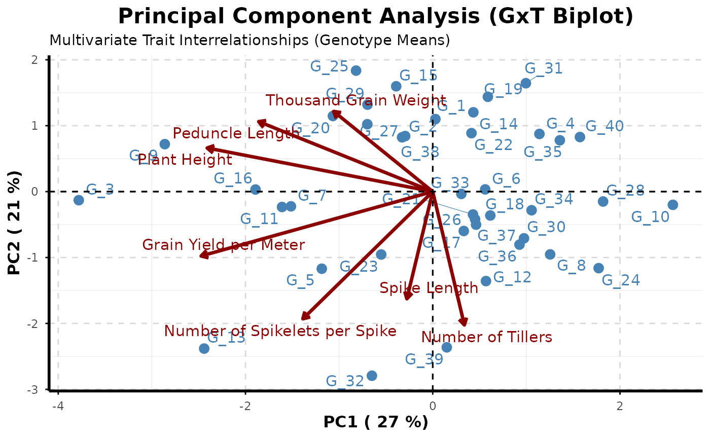
pca_res <- analyze_pca(data = gv_data, traits = traits, trait_lookup = custom_traits_map)
#> =====================================================================================
#> AGRIDATATOOLS PACKAGED ENGINE v0.1.0 - MODERN PCA DECOMPOSITION PIPELINE
#> Analysis Inception: 2026-08-17 12:02:17.343504
#> -------------------------------------------------------------------------------------
#>
#> ---------------------------------------------------------------------------
#> 1. PRINCIPAL COMPONENT EIGENVALUE & VARIANCE SUMMARY (Kaiser Rule)
#> ---------------------------------------------------------------------------
#> Component Eigenvalue Variance_Percent Cumulative_Percent Retain_Kaiser
#> PC1 1.8928 27.0395 27.0395 Yes (EV >= 1)
#> PC2 1.4711 21.0151 48.0546 Yes (EV >= 1)
#> PC3 1.1068 15.8110 63.8656 Yes (EV >= 1)
#> PC4 0.9211 13.1585 77.0241 No
#> PC5 0.6630 9.4719 86.4960 No
#> PC6 0.5910 8.4435 94.9395 No
#> PC7 0.3542 5.0605 100.0000 No
#>
#> ---------------------------------------------------------------------------
#> 2. TRAIT EIGENVECTOR LOADINGS MATRIX
#> ---------------------------------------------------------------------------
#> PC1 PC2 PC3 PC4 PC5 PC6
#> Plant Height -0.5584 0.1740 -0.2200 -0.1935 0.4327 0.2659
#> Spike Length -0.0640 -0.4276 0.6447 -0.2935 -0.0298 0.5568
#> Peduncle Length -0.4309 0.2793 -0.1406 -0.4513 -0.6784 0.0453
#> Number of Tillers 0.0784 -0.5320 -0.1955 -0.6335 0.1333 -0.4970
#> Number of Spikelets per Spike -0.3215 -0.5076 -0.0278 0.4725 -0.4630 -0.1548
#> Thousand Grain Weight -0.2454 0.3200 0.6884 -0.0217 0.0751 -0.5819
#> Grain Yield per Meter -0.5733 -0.2567 -0.0578 0.2182 0.3375 -0.0872
#> PC7
#> Plant Height 0.5605
#> Spike Length -0.0205
#> Peduncle Length -0.2248
#> Number of Tillers 0.0806
#> Number of Spikelets per Spike 0.4203
#> Thousand Grain Weight 0.1370
#> Grain Yield per Meter -0.6580
#>
#> ---------------------------------------------------------------------------
#> 3. TRAIT CONTRIBUTIONS TO COMPONENTS (% Contribution)
#> ---------------------------------------------------------------------------
#> PC1 PC2 PC3 PC4 PC5 PC6 PC7
#> Plant Height 31.18 3.03 4.84 3.75 18.72 7.07 31.41
#> Spike Length 0.41 18.28 41.56 8.62 0.09 31.00 0.04
#> Peduncle Length 18.57 7.80 1.98 20.37 46.02 0.20 5.06
#> Number of Tillers 0.61 28.30 3.82 40.13 1.78 24.70 0.65
#> Number of Spikelets per Spike 10.34 25.76 0.08 22.32 21.43 2.40 17.67
#> Thousand Grain Weight 6.02 10.24 47.39 0.05 0.56 33.87 1.88
#> Grain Yield per Meter 32.87 6.59 0.33 4.76 11.39 0.76 43.29
#> =====================================================================================
#>
plot_agri_graphics(type = "pca", payload = pca_res,
trait_name = "PCA Plot")
#> =====================================================================================
#> AGRIDATATOOLS PACKAGED ENGINE v0.1.0 - INTEGRATED GRAPHICS VISUALIZATION
#> Plot Generation Inception: 2026-08-17 12:02:17.351994
#> -------------------------------------------------------------------------------------
#> [LOG - FINALIZE]: Stream closed in 0.27604 seconds.
# 2. PCA: Multivariate variation
custom_traits_map <- c(
"PH" = "Plant Height",
"SL" = "Spike Length",
"PL" = "Peduncle Length",
"NOT" = "Number of Tillers",
"NOSS" = "Number of Spikelets per Spike",
"TGW" = "Thousand Grain Weight",
"GYPM" = "Grain Yield per Meter"
)
pca_res <- analyze_pca(data = gv_data, traits = traits, trait_lookup = custom_traits_map)
#> =====================================================================================
#> AGRIDATATOOLS PACKAGED ENGINE v0.1.0 - MODERN PCA DECOMPOSITION PIPELINE
#> Analysis Inception: 2026-08-17 12:02:17.343504
#> -------------------------------------------------------------------------------------
#>
#> ---------------------------------------------------------------------------
#> 1. PRINCIPAL COMPONENT EIGENVALUE & VARIANCE SUMMARY (Kaiser Rule)
#> ---------------------------------------------------------------------------
#> Component Eigenvalue Variance_Percent Cumulative_Percent Retain_Kaiser
#> PC1 1.8928 27.0395 27.0395 Yes (EV >= 1)
#> PC2 1.4711 21.0151 48.0546 Yes (EV >= 1)
#> PC3 1.1068 15.8110 63.8656 Yes (EV >= 1)
#> PC4 0.9211 13.1585 77.0241 No
#> PC5 0.6630 9.4719 86.4960 No
#> PC6 0.5910 8.4435 94.9395 No
#> PC7 0.3542 5.0605 100.0000 No
#>
#> ---------------------------------------------------------------------------
#> 2. TRAIT EIGENVECTOR LOADINGS MATRIX
#> ---------------------------------------------------------------------------
#> PC1 PC2 PC3 PC4 PC5 PC6
#> Plant Height -0.5584 0.1740 -0.2200 -0.1935 0.4327 0.2659
#> Spike Length -0.0640 -0.4276 0.6447 -0.2935 -0.0298 0.5568
#> Peduncle Length -0.4309 0.2793 -0.1406 -0.4513 -0.6784 0.0453
#> Number of Tillers 0.0784 -0.5320 -0.1955 -0.6335 0.1333 -0.4970
#> Number of Spikelets per Spike -0.3215 -0.5076 -0.0278 0.4725 -0.4630 -0.1548
#> Thousand Grain Weight -0.2454 0.3200 0.6884 -0.0217 0.0751 -0.5819
#> Grain Yield per Meter -0.5733 -0.2567 -0.0578 0.2182 0.3375 -0.0872
#> PC7
#> Plant Height 0.5605
#> Spike Length -0.0205
#> Peduncle Length -0.2248
#> Number of Tillers 0.0806
#> Number of Spikelets per Spike 0.4203
#> Thousand Grain Weight 0.1370
#> Grain Yield per Meter -0.6580
#>
#> ---------------------------------------------------------------------------
#> 3. TRAIT CONTRIBUTIONS TO COMPONENTS (% Contribution)
#> ---------------------------------------------------------------------------
#> PC1 PC2 PC3 PC4 PC5 PC6 PC7
#> Plant Height 31.18 3.03 4.84 3.75 18.72 7.07 31.41
#> Spike Length 0.41 18.28 41.56 8.62 0.09 31.00 0.04
#> Peduncle Length 18.57 7.80 1.98 20.37 46.02 0.20 5.06
#> Number of Tillers 0.61 28.30 3.82 40.13 1.78 24.70 0.65
#> Number of Spikelets per Spike 10.34 25.76 0.08 22.32 21.43 2.40 17.67
#> Thousand Grain Weight 6.02 10.24 47.39 0.05 0.56 33.87 1.88
#> Grain Yield per Meter 32.87 6.59 0.33 4.76 11.39 0.76 43.29
#> =====================================================================================
#>
plot_agri_graphics(type = "pca", payload = pca_res,
trait_name = "PCA Plot")
#> =====================================================================================
#> AGRIDATATOOLS PACKAGED ENGINE v0.1.0 - INTEGRATED GRAPHICS VISUALIZATION
#> Plot Generation Inception: 2026-08-17 12:02:17.351994
#> -------------------------------------------------------------------------------------
 #> [LOG - FINALIZE]: Stream closed in 0.93767 seconds.
# 3. Clustering: Dendrogram with flexible cluster parameter option
cl_res <- analyze_clustering(data = gv_data, traits = traits, k = k_groups)
#>
#> ===========================================================================
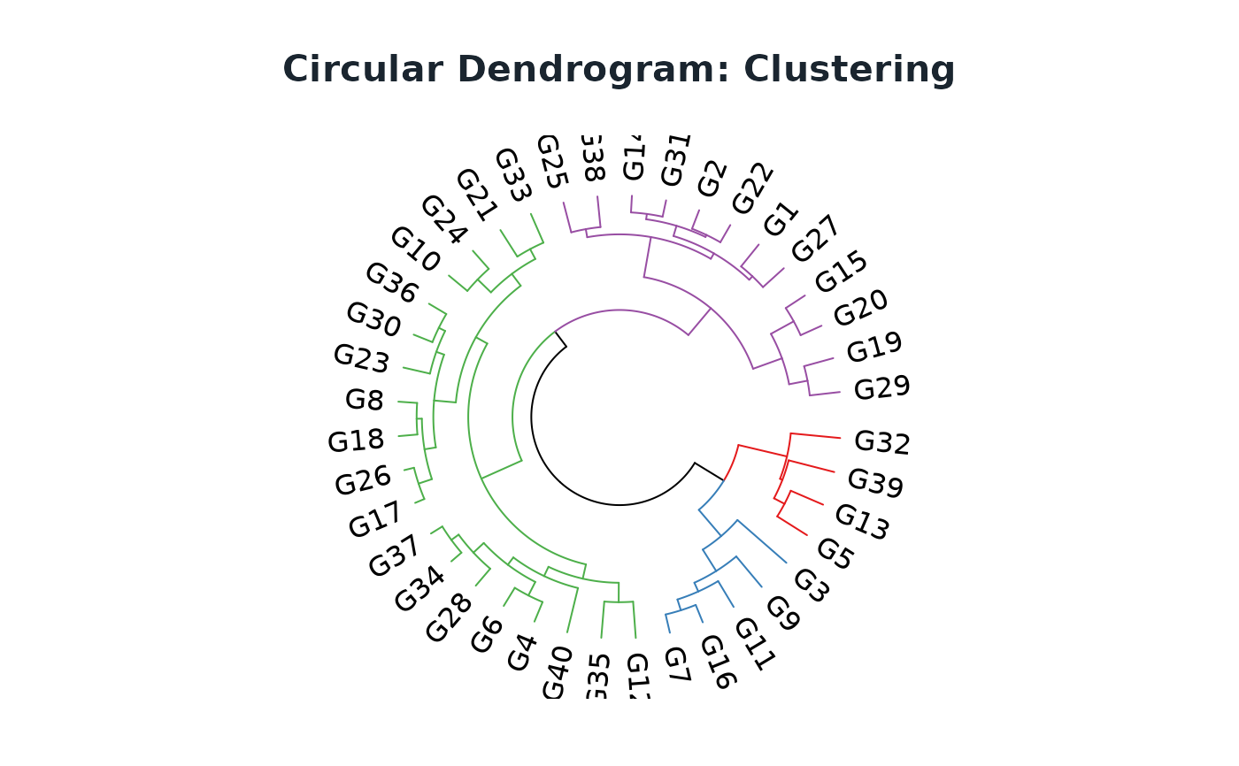
#> HIERARCHICAL CLUSTER ANALYSIS SUMMARY
#> ===========================================================================
#> Linkage Algorithm : ward.D2
#> Total Genotypes Evaluated : 40
#> Number of Clusters (k) : 4
#> Cophenetic Correlation Fit : 0.6204
#> ---------------------------------------------------------------------------
#>
#> --- CLUSTER MEMBERSHIP AND COUNT ---
#> Cluster_1 (n = 12) : G1, G14, G15, G19, G2, G20, G22, G25, G27, G29, G31, G38
#> Cluster_2 (n = 19) : G10, G12, G17, G18, G21, G23, G24, G26, G28, G30, G33, G34, G35, G36, G37, G4, G40, G6, G8
#> Cluster_3 (n = 5) : G11, G16, G3, G7, G9
#> Cluster_4 (n = 4) : G13, G32, G39, G5
#>
#> --- INTRA-CLUSTER DISTANCES (Within Cluster Average) ---
#> Cluster_1 : 2.7456
#> Cluster_2 : 2.6887
#> Cluster_3 : 3.0401
#> Cluster_4 : 3.3706
#>
#> --- INTER-CLUSTER DISTANCE MATRIX (Between Centroids) ---
#> Cluster_1 Cluster_2 Cluster_3 Cluster_4
#> Cluster_1 0.0000 2.2830 3.1488 3.8847
#> Cluster_2 2.2830 0.0000 3.5783 3.2097
#> Cluster_3 3.1488 3.5783 0.0000 3.6038
#> Cluster_4 3.8847 3.2097 3.6038 0.0000
#>
#> --- CLUSTER MEANS MATRIX (Original Trait Values) ---
#> Cluster PH SL PL NOT NOSS TGW GYPM
#> 1 Cluster_1 94.49722 10.48611 26.90278 8.25000 17.67639 36.75472 102.44444
#> 2 Cluster_2 90.42982 11.33333 25.43860 12.38596 18.11421 34.61456 92.49123
#> 3 Cluster_3 100.20000 11.60000 30.93333 12.26667 19.97067 37.66467 134.60000
#> 4 Cluster_4 92.33333 11.54167 26.06667 12.33333 27.30667 32.75667 134.91667
#> ===========================================================================
#>
plot_agri_graphics(type = "cluster", payload = cl_res,
trait_name = "Clustering", num_clusters = k_groups)
#> =====================================================================================
#> AGRIDATATOOLS PACKAGED ENGINE v0.1.0 - INTEGRATED GRAPHICS VISUALIZATION
#> Plot Generation Inception: 2026-08-17 12:02:18.301137
#> -------------------------------------------------------------------------------------
#> [LOG - FINALIZE]: Stream closed in 0.93767 seconds.
# 3. Clustering: Dendrogram with flexible cluster parameter option
cl_res <- analyze_clustering(data = gv_data, traits = traits, k = k_groups)
#>
#> ===========================================================================
#> HIERARCHICAL CLUSTER ANALYSIS SUMMARY
#> ===========================================================================
#> Linkage Algorithm : ward.D2
#> Total Genotypes Evaluated : 40
#> Number of Clusters (k) : 4
#> Cophenetic Correlation Fit : 0.6204
#> ---------------------------------------------------------------------------
#>
#> --- CLUSTER MEMBERSHIP AND COUNT ---
#> Cluster_1 (n = 12) : G1, G14, G15, G19, G2, G20, G22, G25, G27, G29, G31, G38
#> Cluster_2 (n = 19) : G10, G12, G17, G18, G21, G23, G24, G26, G28, G30, G33, G34, G35, G36, G37, G4, G40, G6, G8
#> Cluster_3 (n = 5) : G11, G16, G3, G7, G9
#> Cluster_4 (n = 4) : G13, G32, G39, G5
#>
#> --- INTRA-CLUSTER DISTANCES (Within Cluster Average) ---
#> Cluster_1 : 2.7456
#> Cluster_2 : 2.6887
#> Cluster_3 : 3.0401
#> Cluster_4 : 3.3706
#>
#> --- INTER-CLUSTER DISTANCE MATRIX (Between Centroids) ---
#> Cluster_1 Cluster_2 Cluster_3 Cluster_4
#> Cluster_1 0.0000 2.2830 3.1488 3.8847
#> Cluster_2 2.2830 0.0000 3.5783 3.2097
#> Cluster_3 3.1488 3.5783 0.0000 3.6038
#> Cluster_4 3.8847 3.2097 3.6038 0.0000
#>
#> --- CLUSTER MEANS MATRIX (Original Trait Values) ---
#> Cluster PH SL PL NOT NOSS TGW GYPM
#> 1 Cluster_1 94.49722 10.48611 26.90278 8.25000 17.67639 36.75472 102.44444
#> 2 Cluster_2 90.42982 11.33333 25.43860 12.38596 18.11421 34.61456 92.49123
#> 3 Cluster_3 100.20000 11.60000 30.93333 12.26667 19.97067 37.66467 134.60000
#> 4 Cluster_4 92.33333 11.54167 26.06667 12.33333 27.30667 32.75667 134.91667
#> ===========================================================================
#>
plot_agri_graphics(type = "cluster", payload = cl_res,
trait_name = "Clustering", num_clusters = k_groups)
#> =====================================================================================
#> AGRIDATATOOLS PACKAGED ENGINE v0.1.0 - INTEGRATED GRAPHICS VISUALIZATION
#> Plot Generation Inception: 2026-08-17 12:02:18.301137
#> -------------------------------------------------------------------------------------
 #> [LOG - FINALIZE]: Stream closed in 0.36401 seconds.
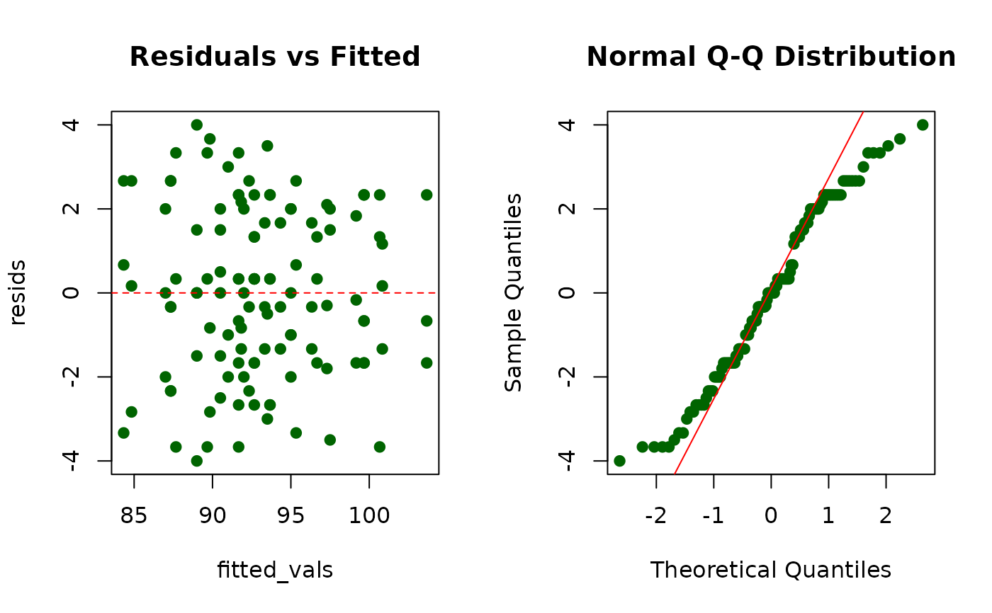
# 4. Residuals: Diagnostic plots
fit <- lm(PH ~ Genotype, data = gv_data)
res_pl <- list(residuals = residuals(fit),
fitted_values = fitted(fit))
plot_agri_graphics(type = "residual", payload = res_pl,
trait_name = "Residuals")
#> =====================================================================================
#> AGRIDATATOOLS PACKAGED ENGINE v0.1.0 - INTEGRATED GRAPHICS VISUALIZATION
#> Plot Generation Inception: 2026-08-17 12:02:18.676431
#> -------------------------------------------------------------------------------------
#> [LOG - FINALIZE]: Stream closed in 0.36401 seconds.
# 4. Residuals: Diagnostic plots
fit <- lm(PH ~ Genotype, data = gv_data)
res_pl <- list(residuals = residuals(fit),
fitted_values = fitted(fit))
plot_agri_graphics(type = "residual", payload = res_pl,
trait_name = "Residuals")
#> =====================================================================================
#> AGRIDATATOOLS PACKAGED ENGINE v0.1.0 - INTEGRATED GRAPHICS VISUALIZATION
#> Plot Generation Inception: 2026-08-17 12:02:18.676431
#> -------------------------------------------------------------------------------------
 #> [LOG - FINALIZE]: Stream closed in 0.01123 seconds.
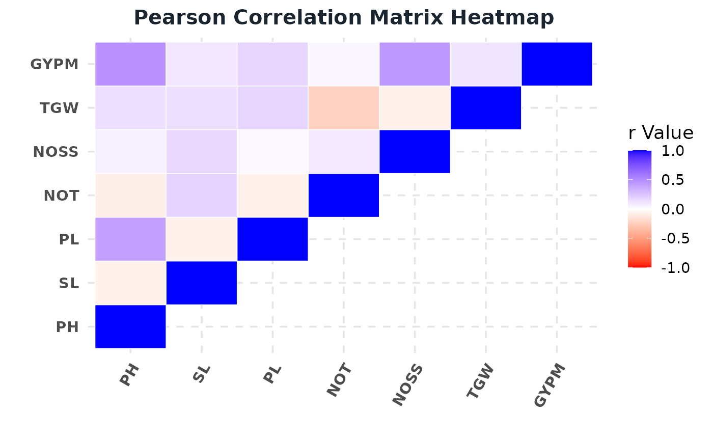
# 5. Correlations: Phenotypic matrix
cor_m <- cor(gv_data[, traits], use = "pairwise.complete.obs")
plot_agri_graphics(type = "correlation",
payload = list(correlation_matrix = cor_m),
trait_name = "Correlation")
#> =====================================================================================
#> AGRIDATATOOLS PACKAGED ENGINE v0.1.0 - INTEGRATED GRAPHICS VISUALIZATION
#> Plot Generation Inception: 2026-08-17 12:02:18.689626
#> -------------------------------------------------------------------------------------
#> [LOG - FINALIZE]: Stream closed in 0.01123 seconds.
# 5. Correlations: Phenotypic matrix
cor_m <- cor(gv_data[, traits], use = "pairwise.complete.obs")
plot_agri_graphics(type = "correlation",
payload = list(correlation_matrix = cor_m),
trait_name = "Correlation")
#> =====================================================================================
#> AGRIDATATOOLS PACKAGED ENGINE v0.1.0 - INTEGRATED GRAPHICS VISUALIZATION
#> Plot Generation Inception: 2026-08-17 12:02:18.689626
#> -------------------------------------------------------------------------------------
 #> [LOG - FINALIZE]: Stream closed in 0.31261 seconds.
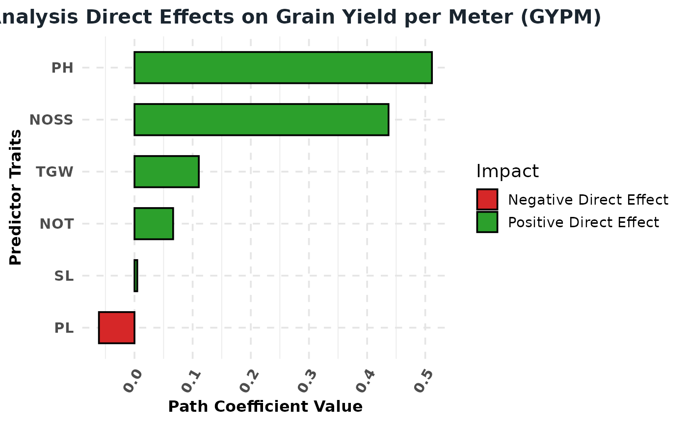
# 6. Path Analysis: Direct Effects Plot for Grain Yield per Meter (GYPM)
corr_res <- compute_correlation(data = gv_data, traits = traits, reporting_level = 0)
all_predictors <- c("PH", "SL", "PL", "NOT", "NOSS", "TGW")
path_res <- compute_path_analysis(
correlation_payload = corr_res,
response_trait = "GYPM",
predictor_traits = all_predictors,
reporting_level = 0
)
plot_agri_graphics(type = "path", payload = path_res, trait_name = "Grain Yield per Meter (GYPM)")
#> =====================================================================================
#> AGRIDATATOOLS PACKAGED ENGINE v0.1.0 - INTEGRATED GRAPHICS VISUALIZATION
#> Plot Generation Inception: 2026-08-17 12:02:19.116357
#> -------------------------------------------------------------------------------------
#> [LOG - FINALIZE]: Stream closed in 0.31261 seconds.
# 6. Path Analysis: Direct Effects Plot for Grain Yield per Meter (GYPM)
corr_res <- compute_correlation(data = gv_data, traits = traits, reporting_level = 0)
all_predictors <- c("PH", "SL", "PL", "NOT", "NOSS", "TGW")
path_res <- compute_path_analysis(
correlation_payload = corr_res,
response_trait = "GYPM",
predictor_traits = all_predictors,
reporting_level = 0
)
plot_agri_graphics(type = "path", payload = path_res, trait_name = "Grain Yield per Meter (GYPM)")
#> =====================================================================================
#> AGRIDATATOOLS PACKAGED ENGINE v0.1.0 - INTEGRATED GRAPHICS VISUALIZATION
#> Plot Generation Inception: 2026-08-17 12:02:19.116357
#> -------------------------------------------------------------------------------------
 #> [LOG - FINALIZE]: Stream closed in 0.22137 seconds.